Finite difference methods value a derivative by solving the differential equation that the derivative satisfies. Consider an American put option on a stock paying a dividend yield of $q$. The associated Black-Scholes equation is:

$$\frac{\partial f}{\partial t} + (r-q)S \frac{\partial f}{\partial S} + \frac{1}{2}\sigma^2 S^2 \frac{\partial^2 f}{\partial S^2} = rf$$

The finite difference method discretizes the time and stock price axis, see Figure below.

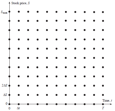
The life of the option is $T$. We divide the time into $N+1$ equally spaced intervals of length $\Delta t = T/N$. For the stock price, we suppose that $S_{max}$ is the max stock price, a price when reached, the put has no value. We divide the stock price into $M+1$ equally spaced intervals of length $\Delta S = S/M$.

The implicit finite difference method discretizes the different partial derivatives such that we get:

$$a_{j}f_{i,j-1} + b_{j}f_{i,j} + c_j f_{i,j+1} = f_{i+1, j}$$

where the coefficients $a_j$, $b_j$ and $c_j$ depends on $r$, $q$, $\Delta t$, $\sigma^2$.

We know the value of the put at time $T$: $max(K-S_T, 0) = f_{N,j}$. We also know its value when the stock price is 0: $f_{i,0}=K$. We assume that its value is worthless when the stock is equal to $S_{max}$.

Therefore, starting from $t=T$ and going backwards, we can solve the value of the derivative on all points in the grid. However, at each time step $t$ we need to not forget to replace the value of $f_{t,j}$ with $K-j\Delta S$ to account for early exercising.

One nice property of the implicit finite difference method is that the user does not have to take any precautions to ensure convergence.

The problem with finite difference methods is that they are difficult to apply when the payoffs depend on the past history of the state variables. They are also liable to become computationally very time consuming when more than three variables are involved.

For more information on finite difference methods, I did a project with D. Duffy here.